Most free GIS programs have a measuring tool that lets you determine the distance between two or more points. But this distance is usually a flat, straight-line distance, and doesn’t take into account the additional distance you would travel if the terrain weren’t flat. If the terrain is steep or hilly, your 3D distance traveled is longer than that flat, straight-line distance.
MicroDEM has the capability to determine both the straight-line distance and distance over terrain for an arbitrary path. After loading in a digital elevation model (DEM), click on the Distance (stream selection) in the window’s toolbar:

Then draw the path on your DEM:

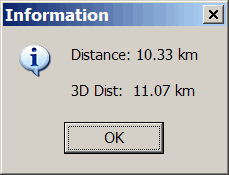
And MicroDEM brings up a window with the flat distance, and 3D distance over terrain:
If you have a map whose area is covered by the DEM, you can draw the path directly on the map:

MicroDEM links the map with the DEM, and will calculate the straight-line and 3D distances:
I’ve been meaning to write about these LIDAR Tools for a while, but since Google Earth Blog has just posted on their Google Earth visualization capabilities, I’ll jump in with my two cents. Posted by Martin Isenburg of the University of North Carolina – Chapel Hill, these tools allow quick conversion of LIDAR data into contour and DEM Google Earth KMZ files for “quick” basic visualization of the data. The process involves taking the original LIDAR data, simplifying it down a bit for contours, then converting it directly to either transparent contour overlays, or high-resolution DEM reflectance overlays. Here’s a screenshot of a set of contours from their showcase overlay gilmer.kmz (click on the image for a larger view):

Note: To see the contours for a grid square, you’ll have to click on the placemark icon for a square, then click on the “load contours” link in the info balloon that pops up.
Here’s a screenshot of the interior of Mt. St. Helens from Google Earth:

And here’s the same view with the high-resolution LIDAR DEM reflectance view loaded in from the saint_helens.kmz file:

All the tools used to create these overlays are downloadable from the website; they’re all command-line tools (ouch), but there’s an example of usage given to make figuring them out a bit easier.
Also available are a basic set of LIDAR tools to:
- Convert text ASCII LIDAR data to the more efficient LAS format
- Print the LIDAR data
- View the LIDAR data
- Compress it losslessly
Download Squad posts that Bryce 5.5, a program that creates photo-realistic landscape renderings and animation with vegetation and realistic skies, is available as a free download (registration required to get a free serial number). While it lets you create your own topography, it also accepts DEMs as input for the landscapes. This is one version below the current 6.1 release, but is still feature-rich. Unfortunately, it also has a very idiosyncratic interface that takes a lot of getting used to. Here’s a review of the program from PC Pro, with some screen shots.
There are other free programs for realistic landscape rendering, with some limitations compared to Bryce 5.5 but also somewhat easier interfaces to navigate:
Genesis IV: Available in a freeware edition for personal use, as well as several paid versions.
Terragen: The free non-commercial version limits the output resolution. There’s also a Technology Preview release of Version 2.0 available as well, though it has a fairly technical interface.
The free program 3DEM can convert a number of DEM formats to Terragen’s native terrain format, and to formats compatible with Genesis IV.
SAGA GIS (System For Automated Geoscientific Analyses) is a free raster/terrain-oriented GIS program (some vector functions), with a modular structure that makes it easy to add additional capabilities. After being in release candidate mode for about a year, the final official version 2.0.0 was released about two weeks ago, replacing the previous version 1.2 stable release. Probably the biggest change is the move from Windows-only to a multi-platform release supporting both Windows and Linux. A quick examination of the module packages shows that a few new modules have been added, but most are unchanged. However, module management has been significantly improved with the addition of a “Modules” tab to the Workspace window, and in general it’s easier to pull up data in the new version.
Best of all, there’s been a huge improvement in documentation. Version 1.2 had a good introductory 200-page manual that’s still worth downloading and reading, but many of the modules had virtually no documentation at all. Version 2.0 now has a terrific 400-page manual, available at the SourceForge download page along with a copy of the demo data used in the manual. And while even the manual doesn’t cover all the functions of the different modules, clicking on a module in the “Modules” window and then clicking on the module’s “Description” tab brings up a cursory description of the module and the input parameters. While it will still take some time to figure the module’s operation out, that’s still better than the way it was with version 1.2. A listing of the available modules is at the bottom of this post, after the fold.
It’s a good thing there are now two good manuals, because program function takes some getting used to. SAGA uses its own raster grid format (.sgrd for version 2.0), so grids in other formats have to be imported into the program (and exported into other formats as well). Setting parameters for individual data layers also takes some getting used to. But given the huge number of module functions available in this program, it’s worth spending some time figuring out how to use it. I hope to cover some of the modules not documented in the manuals in future posts (I’ve already covered using SAGA to convert raster graphics to shapefile format in this post).
A list of modules in SAGA 2.0 follows below the fold (taken from the user manual).
Continue reading ‘SAGA GIS 2.0 Released’
The Viewfinder Panoramas website has an eclectic mix of mountain-related data available. Computer-generated panoramas from the peak of about 200 mountains across the world show the terrain visible from the tops of those peaks, with individual terrain features labeled. Here’s an example, looking north from the top of Mt. Whitney in California (click on the image for a larger view):

The site also has links to DEM terrain data for a number of mountainous regions. Some of it is custom high-resolution data extracted from topo maps, while other datasets are SRTM-90 data with the holes patched using data from topo maps. Areas covered include the Himalayas, Andes and Alps, but scattered data from other areas (e.g. the Canary Islands, Japan) is also available. SRTM-90 data with the holes patched is available from the USGS Seamless Server, but the patching process used there can result in anomalies in the DEMs. The DEMs from the Viewfinder Panorama site appear to be of significantly higher quality than the SRTM-90 data in many cases.
LIDAR (Light Detection and Ranging) can be used to create high-resolution terrain data (sub-meter), detail good enough to show individual man-made features like buildings and bridges. It’s especially useful for analyzing terrain in areas that are in constant change, like coastlines. High-resolution coastal LIDAR data is available at this NOAA website for the entire US ocean coastline, and parts of the Great Lakes coastlines, for times ranging from 1996 to the present.
Continue reading ‘LIDAR Data Coastal Erosion And Flooding Analysis Using MicroDEM’
For general map relief shading, my first choice is usually 3DEM, since it usually gives the best results. But MicroDEM also does a decent job at terrain relief shading, and has a few other shading options that 3DEM lacks.
Continue reading ‘Elevation, Slope, Terrain And 3D Anaglyph Map Shading In MicroDEM’